
Visualizing Apache and ModSecurity Log Files
What are we doing?
We are interpreting the log files visually.
Why are we doing this?
In the preceding tutorials we have customized the Apache log format and performed a variety of statistical analyses. But we have yet to graphically display the numbers obtained. The visualization of data does in fact provide a big help in identifying problems. In particular, time series are very informative and even performance problems can be better quantified and narrowed down visually. But graphical display can also provide interesting information about false positives among the volumes of ModSecurity alarms.
The benefit of visualization is readily apparent and is a good reason why graphs have always been an important component of dashboards and regular reports. However, in this tutorial we will not be aiming for perfectly laid out graphs that management would like. We instead want to get highly informative graphs showing the essential parts of data by the simplest of means possible.
For this reason, we will be using a little-known feature of gnuplot.
Requirements
- An Apache web server, ideally one created using the file structure shown in Tutorial 1 (Compiling an Apache web server).
- Understanding of the minimal configuration in Tutorial 2 (Configuring a minimal Apache server).
- An Apache web server with SSL/TLS support as in Tutorial 4 (Configuring an SSL server)
- An Apache web server with extended access log as in Tutorial 5 (Extending and analyzing the access log)
- An Apache web server with ModSecurity as in Tutorial 6 (Embedding ModSecurity)
- An Apache web server with a Core Rule Set installation as in Tutorial 7 (Embedding Core Rules)
- The
gnuplotpackage; e.g. as present in theUbuntudistribution.
Step 1: Graphically displaying time series in the shell
The appearance of entries in log files follows a chronological sequence. However, it is actually relatively difficult to follow this chronological sequence in the text file. Visualization of the log files is the answer. Dashboards have already been mentioned and a variety of commercial products and open source projects have become established in the past few years. These tools are very useful. But they are not always easily accessible or the log data must first be imported and sometimes even converted or indexed. There is thus a big gap in displaying graphs in the shell. The graphical tool gnuplot can in fact do this in ASCII and be controlled completely from the command line.
gnuplot can be demanding to use and control and if you only use it occasionally you face the same learning curve again and again. For this reason, I have developed a wrapper script called arbigraph that uses gnuplot to display simple graphs: arbigraph We will be using this script in different situations in this tutorial and become familiar with a large number of command line options. So, let’s start off with a simple case:
Let’s generate a simple graph in which the number of requests per hour is presented on a time line. As an example, to do this we are using the access log that we became familiar with while fine tuning ModSecurity false positives in one of the preceding tutorials: tutorial-8-example-access.log.
Let’s concentrate on the entries from May 20 to 29 and extract the timestamps from them:
$> grep 2015-05-2 tutorial-8-example-access.log | altimestamp | head
2015-05-20 12:53:11.139981
2015-05-20 12:53:12.232266
2015-05-20 12:54:57.772135
2015-05-20 12:54:58.842986
2015-05-20 12:54:59.009303
2015-05-20 12:54:59.003103
2015-05-20 12:54:59.006098
2015-05-20 12:54:58.992113
2015-05-20 12:54:58.994096
2015-05-20 12:55:00.270296
Each of these lines represents a request. The number of requests per unit of time can thus be easily determined by counting them. Totaling by hour can be easily done by cutting the timestamp at the colon and adding them up via uniq -c. Just to be safe, we’ll insert a sort since the log files are not necessarily in chronological order (the entry follows the completion of the request, but the timestamp indicates the receipt of the request line in the request. This means that a “slower” request at 12:59 may appear in the log file after a “fast” request at 13:00. We can already see this problem at 12:54:58 and 12:54:59 above).
Here’s the total per hour:
$> grep 2015-05-2 tutorial-8-example-access.log | altimestamp | cut -d: -f1 | sort | uniq -c | head
     37 2015-05-20 12
      6 2015-05-20 13
      1 2015-05-20 14
    105 2015-05-20 15
     38 2015-05-20 16
     25 2015-05-20 17
     19 2015-05-20 18
     32 2015-05-20 19
     19 2015-05-20 22
      1 2015-05-21 06
This seems to work, although there also seem to be gaps in the log file. We’ll be taking care of them later on. In the first column we now see the requests per hour, with the second and third columns showing the time or hour. We now feed the result into the arbigraph script which only uses the first column for graphical display:
$> grep 2015-05-2 tutorial-8-example-access.log | altimestamp | cut -d: -f1 | sort | uniq -c | arbigraph

  250 ++-----------------+-------------------+-------------------+-------------------+-------------------+-------------------++
      |                  +                   +                   +                   +                   +       Col 1 ******+|
      |                                                            **                                                         |
      |                                                            **                                                         |
      |                                                            **                                                         |
  200 ++                                                           **                              **                        ++
      |                                                            **                              **    **                   |
      |                                                            **                              **    **                   |
      |                                                           ***                              **    **       ** **       |
      |                                                           ***                              **    **       ** **       |
  150 ++                        **                                ***            **                ** *****       ** ** **   ++
      |                 **      **                                ***            **                ** *******     ***** **    |
      |                 **      **                                ***            **   **           ** *******     ***** **    |
      |           **    **     ***                                ***            **   **           ** *******     ***** **    |
      |          ***    **     ***                                ***           ***   **  **       ** *******     ***** **    |
  100 ++ **      ***    **     ***                                ***           ***** **  **       ** *******     ***** ***  ++
      |  **      ***    **     ***        **                     ****           ***** **  **       ** *******     *********   |
      |  **     ****   ***     ***        **                     *****          ***** **  **       ** *******     *********   |
      |  **     *****  ***     ***  ***   ** **                  *****          ********  **       **********   ***********   |
      |  **     *****  ***     ***  ***   ** ****                *****          ******** ***       **********   ***********   |
   50 ++ **     **********   ****** ***   *******                *****          ************       **********   ***********  ++
      ** ***    **********   ****** ***   ******* **             *****  **   ** ************       **********   ***********   |
      ** *** ** **********   **********   ******* **        **   *****  ***  ** **************     ************ ************  |
      ** *****************   ********** ********* ****      ** ************* ** **************   **************************** |
      *********************  **************************    *** ********************************  ******************************
    0 *************************************************************************************************************************
                         20                  40                  60                  80                 100                 120
In this rudimentary graphical display we see the number of requests on the y-axis. The timeline is on the x-axis. Peak load is approx. 250 requests per hour. In general, we see the volume of traffic going strongly up and down. At the top right we see the legend which by default the asterisks describe as Col 1. A serious drawback is the useless labeling on the x-axis, since the numbers from 20 to 120 only indicate the line number of the value on the y-axis.
But because we had gaps in the dataset our data is based on, we can no longer infer the time of a value from the number of lines and hence the x-axis in the graph. We’ll first have to close these gaps, then have a closer look at the x-axis problem.
Step 2: Filling in the gaps on the timeline
The problem with the gaps is that for some hours we don’t have a single request in the log file. The log file comes from a server with relatively little traffic. But filtering the log file after an error on a server with significantly more traffic results in gaps appearing in the timeline. We have to close them for good. Up to now we have extracted the date and time from the log file. The approach has proven to be inadequate: Instead of deriving the sequence of dates and hours from the log file, we will be rebuilding it ourselves and looking for the number of requests in the log file for every date and hour combination. A repetitive grep on the same log file would be a bit inefficient, but entirely suitable for the size of the log file in this case. The approach must be optimized for larger files.
$> for DAY in {20..29}; do for HOUR in {00..23}; do echo "2015-05-$DAY $HOUR"; done; done
2015-05-20 00
2015-05-20 01
2015-05-20 02
2015-05-20 03
2015-05-20 04
2015-05-20 05
2015-05-20 06
2015-05-20 07
2015-05-20 08
2015-05-20 09
2015-05-20 10
...
This is our timeline without gaps. Let’s use these values as the basis for a loop and select the number of requests for each value:
$> for DAY in {20..29}; do for HOUR in {00..23}; do echo "2015-05-$DAY $HOUR"; done; done \
| while read STRING; do COUNT=$(grep -c "$STRING" tutorial-8-example-access.log); \
echo "$COUNT $STRING "; done
0 2015-05-20 00
0 2015-05-20 01
0 2015-05-20 02
0 2015-05-20 03
0 2015-05-20 04
0 2015-05-20 05
0 2015-05-20 06
0 2015-05-20 07
0 2015-05-20 08
0 2015-05-20 09
0 2015-05-20 10
0 2015-05-20 11
37 2015-05-20 12
6 2015-05-20 13
1 2015-05-20 14
105 2015-05-20 15
...
We thus read the combined date-hour string in a while loop. We then count the number of requests for each of the strings (via grep -c here) and then output the result along with the date-hour string. This gives us the same result as in the previous example, but this time the gaps are filled in.
Let’s put this output into our graph script.
$> for DAY in {20..29}; do for HOUR in {00..23}; do echo "2015-05-$DAY $HOUR"; done; done \
| while read STRING; do COUNT=$(grep -c "$STRING" tutorial-8-example-access.log); \
echo "$COUNT $STRING "; done | arbigraph

  250 ++-----------------------+------------------------+------------------------+------------------------+------------------++
      |                        +                        +                        +                        +      Col 1 ****** |
      |                                                                            **                                         |
      |                                                                            **                                         |
      |                                                                            **                                         |
  200 ++                                                                           **                     *                  ++
      |                                                                            **                     *  *                |
      |                                                                            **                     *  *                |
      |                                                                            **                     *  *         ***    |
      |                                                                            **                     *  *         ***    |
  150 ++                           **                                              **         **          ****         ****  ++
      |                   *        **                                              **         **          *****        ****   |
      |                   *        **                                              **         ** *        *****        ****   |
      |                *  *        **                                              **         ** *        *****        ****   |
      |               **  *        **                                              **         ** * *      *****        ****   |
  100 ++      *       **  *        **                                              **         **** *      *****        ***** ++
      |       *       **  *        **         *                                   ***         **** *      *****        *****  |
      |       *       ** **        **         *                                   ***         **** *      *****        *****  |
      |       *       *****        ****       ***                                 ***         **** *      *****       ******  |
      |       *       *****        ****       ****                                ***         ******      *****       ******  |
   50 ++      *       *****       *****       ****                                ***         ******      *****       ****** ++
      |     ****      *****       *****       ******                              *** *  *    ******      *****       ******  |
      |     *****     *****       *****       ******                       *      *** ** *    *******     ******      ******  |
      |     *******   *****       ***** **    ****** *                     *     ******* *    *******  **********     ******* |
      |     *******   ******   +  ********    ****** ** +                 **     **********   ******** **********     ********|
    0 ++----*******--*********-+--********----******-**-+--**--*-----*********---***********--*******************-----********+
                               50                      100                      150                      200
There now appears to be a degree of regularity, because every 24 values is an entire day. Knowing this, we see the daily rhythm, can surmise Saturday and Sunday and may even see indications of a specific lunch break.
Step 3: X-axis label
The gaps are closed. Let’s get to the specific labeling of the x-axis. arbigraph is able to read labels from the input. It identifies the labels on its own; but for this purpose they must be separated by a tab from the actual data. echo does this for us when we set the escape flag
$> for DAY in {20..29}; do for HOUR in {00..23}; do echo "2015-05-$DAY $HOUR"; done; done \
| while read STRING; do COUNT=$(grep -c "$STRING" tutorial-8-example-access.log); \
echo -e "$STRING\t$COUNT"; done | arbigraph

  250 +++++++++++++++++++++++++++++++++++++++++++++++++++++++++++++++++++++++++++++++++++++++++++++++++++++++++++++++++++++++++
      +++++++++++++++++++++++++++++++++++++++++++++++++++++++++++++++++++++++++++++++++++++++++++++++++++++++++++Col 1+******++
      |                                                                            **                                         |
      |                                                                            **                                         |
      |                                                                            **                     *                   |
  200 ++                                                                           **                     *                  ++
      |                                                                            **                     *                   |
      |                                                                            **                     *             **    |
      |                                                                            **                     *             **    |
  150 ++                           **                                              **         **          ****          ***  ++
      |                   *        **                                              **         **          *****        ****   |
      |                   *        **                                              **         ** *        *****        ****   |
      |                *  *        **                                              **         ** *        *****        ****   |
      |               **  *        **                                              **         ** *        *****        ****   |
  100 ++              **  *        **         *                                   ***         ****        *****        ***** ++
      |               ** **        **         *                                   ***         ****        *****        *****  |
      |               ** **        ****       *                                   ***         ****        *****        *****  |
      |               *****        ****       ***                                 ***         ****        *****       ******  |
   50 ++              *****        ****       ****                                ***         ******      *****       ****** ++
      |               *****       *****       ******                              ***         ******      *****       ******  |
      |     *****     *****       *****       ******                       *      *** *       *******     *****       ******  |
      |     *******   *****  *    ****** **   *********         *          ***    ****** *    ******************* *   ******* |
      +++++********++*******+*++++*********+++*********++++*+**+*++++++**+****+++**********+++*******************+*+++********+
    0 +++*+*********+*********+**+*********+*+*********+**+******++++*********+*+************+*******************+*+**********+
    20150151501515015150151501515015150151501515015150151501515015150151501515015150151501515015150151501515015150151501515015
      -  - -  - -  - -  - -  - -  - -  - -  - -  - -  - -  - -  - -  - -  - -  - -  - -  - -  - -  - -  - -  - -  - -  - -  -
    05-20-2020-2020-2121-2121-2122-2222-2222-2323-2323-2324-2424-2425-2525-2525-2626-2626-2627-2727-2727-2828-2828-2829-2929-29
The labels are there, but they are clearly too close together and overlap one another. We have to find a remedy here. One option with the cumbersome name of --xaxisticsmodulo enables us to now write every nth x-axis value. Every 24th value would add one label per day:
$> for DAY in {20..29}; do for HOUR in {00..23}; do echo "2015-05-$DAY $HOUR"; done; done \
| while read STRING; do COUNT=$(grep -c "$STRING" tutorial-8-example-access.log); \
echo -e "$STRING\t$COUNT"; done | arbigraph --xaxisticsmodulo 24


  250 +++++++++++++++++++++++++++++++++++++++++++++++++++++++++++++++++++++++++++++++++++++++++++++++++++++++++++++++++++++++++
      +++++++++++++++++++++++++++++++++++++++++++++++++++++++++++++++++++++++++++++++++++++++++++++++++++++++++++Col 1+******++
      |                                                                            **                                         |
      |                                                                            **                                         |
      |                                                                            **                     *                   |
  200 ++                                                                           **                     *  *               ++
      |                                                                            **                     *  *                |
      |                                                                            **                     *  *         ***    |
      |                                                                            **                     *  *         ***    |
  150 ++                           **                                              **         **          ****         ****  ++
      |                   *        **                                              **         **          *****        ****   |
      |                   *        **                                              **         ** *        *****        ****   |
      |                *  *        **                                              **         ** *        *****        ****   |
      |       *       **  *        **                                              **         ** * *      *****        ****   |
  100 ++      *       **  *        **         *                                   ***         **** *      *****        ***** ++
      |       *       ** **        **         *                                   ***         **** *      *****        *****  |
      |       *       ** **        ****       *                                   ***         **** *      *****        *****  |
      |       *       *****        ****       ***                                 ***         **** *      *****       ******  |
   50 ++      *       *****        ****       ****                                ***         ******      *****       ****** ++
      |       *       *****       *****       ******                              ***    *    ******      *****       ******  |
      |     *****     *****       *****       ******                       *      *** ** *    *******     *****       ******  |
      |     *******   *****  **   *****  **   ****** **          **        * **  ******* **   *********************   *********
      ++++++*******+++******+**+++*********+++******+**++++++++++**+++++++**+**++**********+++*********************+++*********
    0 ++++++*******++**********+++*********+++******+**++++**++*+**++**********++***********++*********************+++*********
               2015        2015        2015        2015        2015        2015        2015        2015        2015        2015
                 -           -           -           -           -           -           -           -           -           -
               05-20       05-21       05-22       05-23       05-24       05-25       05-26       05-27       05-28       05-29
We are getting closer to the goal. What’s still problematic is that the date-hour combination is wrapped at the hyphen and the hours are completely missing. If we replace the hyphen, this wrapping will no longer occur. Let’s have sed help us out.
$> for DAY in {20..29}; do for HOUR in {00..23}; do echo "2015-05-$DAY $HOUR"; done; done \
| while read STRING; do COUNT=$(grep -c "$STRING" tutorial-8-example-access.log); \
echo -e "$STRING\t$COUNT"; done | sed -e "s/-/./g" | arbigraph --xaxisticsmodulo 24


  250 +++++++++++++++++++++++++++++++++++++++++++++++++++++++++++++++++++++++++++++++++++++++++++++++++++++++++++++++++++++++++
      +++++++++++++++++++++++++++++++++++++++++++++++++++++++++++++++++++++++++++++++++++++++++++++++++++++++++++Col 1+******++
      |                                                                            **                                         |
      |                                                                            **                                         |
      |                                                                            **                     *                   |
  200 ++                                                                           **                     *  *               ++
      |                                                                            **                     *  *                |
      |                                                                            **                     *  *         ***    |
      |                                                                            **                     *  *         ***    |
  150 ++                           **                                              **         **          ****         ****  ++
      |                   *        **                                              **         **          *****        ****   |
      |                   *        **                                              **         ** *        *****        ****   |
      |                *  *        **                                              **         ** *        *****        ****   |
      |       *       **  *        **                                              **         ** * *      *****        ****   |
  100 ++      *       **  *        **         *                                   ***         **** *      *****        ***** ++
      |       *       ** **        **         *                                   ***         **** *      *****        *****  |
      |       *       ** **        ****       *                                   ***         **** *      *****        *****  |
      |       *       *****        ****       ***                                 ***         **** *      *****       ******  |
   50 ++      *       *****        ****       ****                                ***         ******      *****       ****** ++
      |       *       *****       *****       ******                              ***    *    ******      *****       ******  |
      |     *****     *****       *****       ******                       *      *** ** *    *******     *****       ******  |
      |     *******   *****  **   *****  **   ****** **          **        * **  ******* **   *********************   *********
      ++++++*******+++******+**+++*********+++******+**++++++++++**+++++++**+**++**********+++*********************+++*********
    0 ++++++*******++**********+++*********+++******+**++++**++*+**++**********++***********++*********************+++*********
            2015.05.20  2015.05.21  2015.05.22  2015.05.23  2015.05.24  2015.05.25  2015.05.26  2015.05.27  2015.05.28  2015.05.29
Now only the hours are still not visible. As can be seen further above, they are separated by a space from the date. If we replace this space by a hyphen then be get a word wrap between the date and the hour.
$> for DAY in {20..29}; do for HOUR in {00..23}; do echo "2015-05-$DAY $HOUR"; done; done \
| while read STRING; do COUNT=$(grep -c "$STRING" tutorial-8-example-access.log); \
echo -e "$STRING\t$COUNT"; done | sed -e "s/-/./g" -e "s/ /-/" | arbigraph --xaxisticsmodulo 24
  250 +++++++++++++++++++++++++++++++++++++++++++++++++++++++++++++++++++++++++++++++++++++++++++++++++++++++++++++++++++++++++
      +++++++++++++++++++++++++++++++++++++++++++++++++++++++++++++++++++++++++++++++++++++++++++++++++++++++++++Col 1+******++
      |                                                                            **                                         |
      |                                                                            **                                         |
      |                                                                            **                     *                   |
  200 ++                                                                           **                     *  *               ++
      |                                                                            **                     *  *                |
      |                                                                            **                     *  *         ***    |
      |                                                                            **                     *  *         ***    |
  150 ++                           **                                              **         **          ****         ****  ++
      |                   *        **                                              **         **          *****        ****   |
      |                   *        **                                              **         ** *        *****        ****   |
      |                *  *        **                                              **         ** *        *****        ****   |
      |       *       **  *        **                                              **         ** * *      *****        ****   |
  100 ++      *       **  *        **         *                                   ***         **** *      *****        ***** ++
      |       *       ** **        **         *                                   ***         **** *      *****        *****  |
      |       *       ** **        ****       *                                   ***         **** *      *****        *****  |
      |       *       *****        ****       ***                                 ***         **** *      *****       ******  |
   50 ++      *       *****        ****       ****                                ***         ******      *****       ****** ++
      |       *       *****       *****       ******                              ***    *    ******      *****       ******  |
      |     *****     *****       *****       ******                       *      *** ** *    *******     *****       ******  |
      |     *******   *****       *****  *    ****** *                     *     ******* *    *******  **********     ******* |
      ++++++*******+++******++++++********++++******+**+++++++++++++++++++**+++++**********+++********+**********+++++********+
    0 ++++++*******++*********++++********++++******+**++++**++*+++++*********+++***********++*******************+++++********+
            2015.05.20  2015.05.21  2015.05.22  2015.05.23  2015.05.24  2015.05.25  2015.05.26  2015.05.27  2015.05.28  2015.05.29
                 -           -           -           -           -           -           -           -           -           -
                22          22          22          22          22          22          22          22          22          22
We will now label the x-axis with every 24th value and by chance we get only to the 22nd hour. We should shift it. Ideally, the middle of each day as well as the 12th hour should be labeled. We can specify such a shift using the --xaxisticsmodulo option. This is done as follows:
$> for DAY in {20..29}; do for HOUR in {00..23}; do echo "2015-05-$DAY $HOUR"; done; done \
| while read STRING; do COUNT=$(grep -c "$STRING" tutorial-8-example-access.log); \
echo -e "$STRING\t$COUNT"; done | sed -e "s/-/./g" -e "s/ /-/" | arbigraph --xaxisticsmodulo 24/10 -w 130


  250 +++++++++++++++++++++++++++++++++++++++++++++++++++++++++++++++++++++++++++++++++++++++++++++++++++++++++++++++++++++++++
      +++++++++++++++++++++++++++++++++++++++++++++++++++++++++++++++++++++++++++++++++++++++++++++++++++++++++++Col 1+******++
      |                                                                            **                                         |
      |                                                                            **                                         |
      |                                                                            **                     *                   |
  200 ++                                                                           **                     *  *               ++
      |                                                                            **                     *  *                |
      |                                                                            **                     *  *         ***    |
      |                                                                            **                     *  *         ***    |
  150 ++                           **                                              **         **          ****         ****  ++
      |                   *        **                                              **         **          *****        ****   |
      |                   *        **                                              **         ** *        *****        ****   |
      |                *  *        **                                              **         ** *        *****        ****   |
      |       *       **  *        **                                              **         ** * *      *****        ****   |
  100 ++      *       **  *        **         *                                   ***         **** *      *****        ***** ++
      |       *       ** **        **         *                                   ***         **** *      *****        *****  |
      |       *       ** **        ****       *                                   ***         **** *      *****        *****  |
      |       *       *****        ****       ***                                 ***         **** *      *****       ******  |
   50 ++      *       *****        ****       ****                                ***         ******      *****       ****** ++
      |       *       *****       *****       ******                              ***    *    ******      *****       ******  |
      |     *****     *****       *****       ******                       *      *** ** *    *******     *****       ******  |
      |     *******   *****       *****  *    ****** *                     *     ******* *    *******  **********     ******* |
      ++++++*******+++******++++++********++++******+**+++++++++++++++++++**+++++**********+++********+**********+++++********+
    0 ++++++*******++*********++++********++++******+**++++**++*+++++*********+++***********++*******************+++++********+
       2015.05.20  2015.05.21  2015.05.22  2015.05.23  2015.05.24  2015.05.25  2015.05.26  2015.05.27  2015.05.28  2015.05.29
            -           -           -           -           -           -           -           -           -           -
           12          12          12          12          12          12          12          12          12          12
We can use a number value after a slash to shift the labeled value to the left or right. Whole positive and negative values are allowed for this.
This gives use the desired graph. One detail are the many plus signs in the top and bottom borders of the graph. They are related to the large number of (hidden) labels and disrupt the picture a bit. I will try to suppress them in a future version of this tutorial.
Step 4: Additional labels
arbigraph provides some options for influencing graphs. Let’s have a look at the options:
$> arbigraph -h

<STDIN> | arbigraph [OPTIONS]

A script to plot a simple graph

 -c  --columnnames STR     Name for columns. Separate by ';'.
 -C  --custom STR          Custom arbitrary gnuplot directives; will be placed right
                           before the plot directive. Separate commands with semicolon.
 -d  --dots                Graph with dots instead of blocks
 -e  --enablescript        Output the gnuplot script below the graph and keep data file
 -h  --help                This text
 -H  --height  STR         Graph height in characters
 -l  --lines               Graph with lines instead of blocks
     --label               Additional text inside the graph. Default positioned top left
 -L  --logscale            Logarithmic scale. Default is normal scale.
 -m  --minx STR            Starting value of x-axis. Default is 1
 -o  --output STR          Write graph into a file (png)
 -s  --sameaxis            Use the same y-axis. Default is separate axis
 -t  --title STR           Title of graph
 -w  --width STR           Width of graph (terminal actually). Default is terminal width
 -x  --xaxisticsmodulo N   Suppress labels on certain tics on the x axis. xaxisticsmodulo 5
                           means every Nth tics gets a label. Default is 5. 1 means
                           every tics gets a label.
 -2                        Use an additional, second data column

Example:
 ls -l /tmp | head -15 | grep -v total | awk '{ print $5 " " $9 } ' | arbigraph

Arbigraph will graph the first column. Subsequent columns are ignored.
The X-axis is actually the line number of a value.
Command line option "minx" therefore defines the
starting point of the line numbering.

A label inside the graph can be added with the --label option. By default, this is
is put in the top left corner. You can align it to the right by adding "(right)"
inside the label text. This will not be printed. You can use \n to get a CR:
$> arbigraph --label '\n\n\n                  PEAK--->'

The caption (tics) on the x axis are always crowded. Use --xaxisticsmodulo to
suppress some of the labels. A value of 5 means, that only every 5th label is
printed. The other ones are hidden.
You can define an offset for the first label to be printed. So that no the 5th
starting from 0 will be printed, but the 5th starting from 2. Define this shift
behind a slash. Negative values are ok.
$> arbigraph --xaxisticsmodulo "24/-2"
You will have to try out various values for xaxisticsmodulo and a shift to the
right or to the left until you find something that suits the data and the graph.
We can thus use --columnnames to add a legend and perhaps also a title using --title. To try out other display options, it is advisable to with --lines:
$> for DAY in {20..29}; do for HOUR in {00..23}; do echo "2015-05-$DAY $HOUR"; done; done \
| while read STRING; do COUNT=$(grep -c "$STRING" tutorial-8-example-access.log);\
echo -e "$STRING\t$COUNT"; done | sed -e "s/-/./g" -e "s/ /-/"\
| arbigraph -x 24/10 --columnnames "Num of Reqs/h" \
--title "Daily Rhythm of Requests in tutorial-8-example-access.log" --lines


                                       Daily Rhythm of Requests in tutorial-8-example-access.log

  250 +++++++++++++++++++++++++++++++++++++++++++++++++++++++++++++++++++++++++++++++++++++++++++++++++++++++++++++++++++++++++
      |++++++++++++++++++++++++++++++++++++++++++++++++++++++++++++++++++++++++++++++++++++++++++++++++++Num of Reqs/h+******++
      |                                                                             *                                         |
      |                                                                             *                                         |
      |                                                                             *                     *                   |
  200 ++                                                                           **                     *  *               ++
      |                                                                            **                     *  *                |
      |                                                                            **                     *  **        * *    |
      |                                                                            **                     *  **        ***    |
  150 ++                            *                                              **          *          * ***        ****  ++
      |                   *         *                                              **          * *        *****        ****   |
      |                   *        **                                              **         ** *        *** *        *****  |
      |                *  *        **                                              **         ** * *      *** *        * ***  |
  100 ++      *        *  *        **                                              **         **** *      *** *        * *** ++
      |       *       * * *        **         *                                    **         ******      *** *        * ***  |
      |       *       * * *        **         *                                    **         ******      **   *       * ***  |
      |       **      * * **       ** *       ***                                  **         ******      **   *      ** ***  |
      |       **      * * **       ** *       ****                                 **         *** ***     **   *      *   **  |
   50 ++      **      * ****      *** *       **** *                              *  *   *    *   ***     **   *      *   ** ++
      |      ****     *  * *      *  * *      **** *                       *      *  *** *    *   ***     **   *      *   **  |
      |      **** *   *  * *      *  * * *    *  *** *                     *      *  *** **   *   * **  * *    **     *   **  |
      |+++++***++**+++*++*+*++++++*++++****+++*++***+**++++++++++++++++++++**+++++*+++++***+++*+++*+**++*+*+++++**++++*+++++**+
    0 +******+*++******++++********+++++*******++**+***********************+******++++++*******++++++*****+++++++******+++++***
        2015.05.20  2015.05.21  2015.05.22  2015.05.23  2015.05.24  2015.05.25  2015.05.26  2015.05.27  2015.05.28  2015.05.29
             -           -           -           -           -           -           -           -           -           -
            12          12          12          12          12          12          12          12          12          12
This eventually takes us to the limits of arbigraph’s capabilities. For gnuplot itself, on which it is based, it is still far from the end of the story. We can issue additional gnuplot commands via the --custom option. Or use --enablescript and have the gnuplot script displayed to us:
for DAY in {20..29}; do for HOUR in {00..23}; do echo "2015-05-$DAY $HOUR"; done; done\
| while read STRING; do COUNT=$(grep -c "$STRING" tutorial-8-example-access.log);\
echo -e "$STRING\t$COUNT"; done | sed -e "s/-/./g" -e "s/ /-/" \
| arbigraph -x 24/10 --columnnames "Num of Reqs/h" \
--title "Daily Rhythm of Requests in tutorial-8-example-access.log" --lines --enablescript

...

THE GNUPLOT SCRIPT
------------------
set terminal dumb 130 30 ;  set boxwidth 1; set format x "\n\n"; set title "Daily Rhythm of Requests in tutorial-8-example-access.log"; ;; ; ;  plot [1:241][0:253] "/tmp/arbigXBwhcT.data" using 1:3:xtic(2) title "Num of Reqs/h" with lines

The transformed data file /tmp/arbigXBwhcT.data is left for future use.
We can copy the script into a text file and pass it to gnuplot as STDIN. This works because the data file which arbigraph wrote for gnuplot in gnuplot data format was saved for further use (/tmp/arbigXBwhcT.data in this case).
$> cat gnuplot-script.gp | gnuplot
                                       Daily Rhythm of Requests in tutorial-8-example-access.log

  250 +++++++++++++++++++++++++++++++++++++++++++++++++++++++++++++++++++++++++++++++++++++++++++++++++++++++++++++++++++++++++
      |++++++++++++++++++++++++++++++++++++++++++++++++++++++++++++++++++++++++++++++++++++++++++++++++++Num of Reqs/h+******++
      |                                                                             *                                         |
      |                                                                             *                                         |
      |                                                                             *                     *                   |
  200 ++                                                                           **                     *  *               ++
      |                                                                            **                     *  *                |
      |                                                                            **                     *  **        * *    |
      |                                                                            **                     *  **        ***    |
  150 ++                            *                                              **          *          * ***        ****  ++
      |                   *         *                                              **          * *        *****        ****   |
      |                   *        **                                              **         ** *        *** *        *****  |
      |                *  *        **                                              **         ** * *      *** *        * ***  |
  100 ++      *        *  *        **                                              **         **** *      *** *        * *** ++
      |       *       * * *        **         *                                    **         ******      *** *        * ***  |
      |       *       * * *        **         *                                    **         ******      **   *       * ***  |
      |       **      * * **       ** *       ***                                  **         ******      **   *      ** ***  |
      |       **      * * **       ** *       ****                                 **         *** ***     **   *      *   **  |
   50 ++      **      * ****      *** *       **** *                              *  *   *    *   ***     **   *      *   ** ++
      |      ****     *  * *      *  * *      **** *                       *      *  *** *    *   ***     **   *      *   **  |
      |      **** *   *  * *      *  * * *    *  *** *                     *      *  *** **   *   * **  * *    **     *   **  |
      |+++++***++**+++*++*+*++++++*++++****+++*++***+**++++++++++++++++++++**+++++*+++++***+++*+++*+**++*+*+++++**++++*+++++**+
    0 +******+*++******++++********+++++*******++**+***********************+******++++++*******++++++*****+++++++******+++++***
        2015.05.20  2015.05.21  2015.05.22  2015.05.23  2015.05.24  2015.05.25  2015.05.26  2015.05.27  2015.05.28  2015.05.29
             -           -           -           -           -           -           -           -           -           -
            12          12          12          12          12          12          12          12          12          12
Provided you have sufficient expertise in using gnuplot, you can now carry on and generate a “report-ready” graph.
Step 5: Graphically displaying a value distribution in the shell
Besides time series, our arbigraph combined with gnuplot can also visually render the distribution of values. Let’s look for example at the duration value documented in the different requests.
$> head -10 tutorial-8-example-access.log | alduration
935006
867783
991977
985790
981818
1001088
1000670
1048915
1057174
826016
What we find here is on the order of 1 million microseconds. How does that look statistically (we are still familiar with the routines from earlier tutorials)?
$> cat tutorial-8-example-access.log | alduration | basicstats.awk
Num of values:        10000
      Average:      2531653
       Median:      1080252
          Min:          688
          Max:     72941899
        Range:     72941211
Std deviation:      5794915
This is apparently a slow application and there are also a lot of outliers towards the top.
We have 10,000 individual data points in the log file. Let’s map them. Because the values are so far apart we choose a logarithmic scale for the y-axis. The graph should be based on lines. Because we are working with 10,000 data points, it may take a moment to draw it:
$> cat tutorial-8-example-access.log  | alduration  | arbigraph --lines --logscale


         +----------------------+-----------*-----------+----------*-----------+-----------------------+----------------------+
         +                      +         *** ***** *  *+         ***          +   ***                 +         Col 1 ****** +
         +                                *** ***** *  *         ****              ***                                        +
   1e+07 ++               *            *  *** ***** *  *     *   ****            *****     *                                 ++
         +*   *    **   * *** ** **   **  *** ***** * **     *   *****          ******   * *   *  * *     *        **   * *   +
         **********************************************************************************************************************
   1e+06 **********************************************************************************************************************
         ************************************* **************** ************************** **** ******************************+
         *** *   *  ***    **** * ** *  * ***  **** **** * **   * ***  ****  * *** ******  ****   ***** ** * *  * ****     * *+
  100000 *** *   *  ***    **** * ** *  * ***  **** **** * **   * ***  ****  * *** ******  ****   ***** ** * *  * ****     * *+
         *** *   *  ***    **** * ** *  * ***  **** **** * **   * ***  ****  * *** ******  ****   ***** ** * *  * ****     * *+
         *** *   *  ***    **** * ** *  * ***  **** **** * **   * ***  ****  * *** ******  ****   ***** ** * *  * ****     * *+
   10000 *** *   *  ***    **** * ** *  * ***  **** **** * **   * ***  ****  * *** ******  ****   ***** ** * *  * ****     * *+
         +** *   *  ***    **** * ** *  * ***  **** **** * **   * ***  ****  * *** ******  ****   ***** ** * *  * ****     * *+
         |** *   *  **     * ** * ** *  * **   **** **** *  *   * ***  ****  * **  ** ***  ****   *** * **      *  ***     *  |
         +   *       *            *  *            *   **                *    *     *        *     ***   *                     +
    1000 ++  *                                        *                                                                      ++
         |                                                                                                                    |
         +                                                                                                                    +
     100 ++                                                                                                                  ++
         +                                                                                                                    +
         +                                                                                                                    +
      10 ++                                                                                                                  ++
         +                                                                                                                    +
         +                      +                       +                      +                       +                      +
       1 ++---------------------+-----------------------+----------------------+-----------------------+---------------------++
         0                     2000                    4000                   6000                    8000                  10000
We used the command above to replace the blocks with lines and used a logarithmic scale, because the outliers were optically too dominant. The graph is however not really satisfactory. The reason is the excessive number of data points. Our terminal has only 80, 120 or, in extreme cases, 200 columns. This is of course too few for a set with 10,000 points, which is why gnuplot itself transfers the graph in relatively few data series. Outliers are centered and smoothed out. Then comes the familiar problem with the badly labeled x-axis.
What we are lacking is a method called binning in statistics. The term binning means summarizing data series into a group. A typical example is a statistic that states that of 20-29 year-olds 45% blah blah and of 30-39 year-olds only 28% blah blah. For 40-40 year-olds… The bins here are the 10-year age groups. The width of the bin can be freely chosen and the content of the bin is then a compilation of the values. In our case, we subdivide the durations of requests into individual bins and for each bin count how many requests there were in this group or this bin.
There is a tool available for performing this binning process: do-binning.rb.
$> cat tutorial-8-example-access.log | alduration | do-binning.rb --label
688.0-3647748.6 9221
3647748.6-7294809.1     180
7294809.1-10941869.6    106
10941869.6-14588930.2   57
14588930.2-18235990.8   65
18235990.8-21883051.3   51
21883051.3-25530111.8   47
25530111.8-29177172.4   32
29177172.4-32824233.0   175
32824233.0-36471293.5   20
36471293.5-40118354.1   22
40118354.1-43765414.6   10
43765414.6-47412475.2   5
47412475.2-51059535.7   2
51059535.7-54706596.3   1
54706596.3-58353656.8   1
58353656.8-62000717.4   2
62000717.4-65647777.9   2
65647777.9-69294838.5   0
69294838.5-72941899.0   0
72941899.0-infinity     1
In the first column we see the width of the bin, the lower and upper end, and next to it in the second column the number of requests in this bin. The bins were defined by the script itself and that’s were the problem with this result lies. Everything is relatively random. Let’s try it with cleanly defined bins and cut off at 2.5 seconds; everything else is an outlier anyway:
$> cat tutorial-8-example-access.log | alduration | do-binning.rb --label -n 25 --min 0 --max 2500000.0
0.0-100000.0    150
100000.0-200000.0       0
200000.0-300000.0       0
300000.0-400000.0       0
400000.0-500000.0       14
500000.0-600000.0       54
600000.0-700000.0       188
700000.0-800000.0       367
800000.0-900000.0       1182
900000.0-1000000.0      1862
1000000.0-1100000.0     1423
1100000.0-1200000.0     1024
1200000.0-1300000.0     706
1300000.0-1400000.0     525
1400000.0-1500000.0     371
1500000.0-1600000.0     306
1600000.0-1700000.0     238
1700000.0-1800000.0     168
1800000.0-1900000.0     136
1900000.0-2000000.0     82
2000000.0-2100000.0     72
2100000.0-2200000.0     68
2200000.0-2300000.0     54
2300000.0-2400000.0     40
2400000.0-2500000.0     39
This looks a lot better. We feed this result into the graph script (and clarify right off that we don’t want to have each value labeled); we saw how this works above.
$> cat tutorial-8-example-access.log | alduration | do-binning.rb --label -n 25 --min 0 --max 2500000.0 \
| arbigraph --xaxisticsmodulo 5/3


  2000 +++----+---+----+----+---+----+---+----+---+----+----+---+----+---+----+----+---+----+---+----+---+----+----+---+----+++
       | +    +   +    +    +   +    +   +    +   +    +    +   +    +   +    +    +   +    +   +    +   +    +  Col 1 ****** |
  1800 ++                                       ******                                                                       ++
       |                                        *    *                                                                        |
       |                                        *    *                                                                        |
  1600 ++                                       *    *                                                                       ++
       |                                        *    *                                                                        |
  1400 ++                                       *    *****                                                                   ++
       |                                        *    *   *                                                                    |
  1200 ++                                   *****    *   *                                                                   ++
       |                                    *   *    *   *                                                                    |
  1000 ++                                   *   *    *   ******                                                              ++
       |                                    *   *    *   *    *                                                               |
       |                                    *   *    *   *    *                                                               |
   800 ++                                   *   *    *   *    *                                                              ++
       |                                    *   *    *   *    ******                                                          |
   600 ++                                   *   *    *   *    *    *                                                         ++
       |                                    *   *    *   *    *    *****                                                      |
   400 ++                                   *   *    *   *    *    *   *                                                     ++
       |                               ******   *    *   *    *    *   **********                                             |
       |                               *    *   *    *   *    *    *   *    *   ******                                        |
   200 ******                     ******    *   *    *   *    *    *   *    *   *    **********                              ++
       * +  * +   +    +    + *****  + * +  * + * +  * + *  + * +  * + * +  * + *  + * + *  + *******************  +   +    + |
     0 ******-+---+----+-*************************************************************************************************--+++
        0.0                 500000.0               1000000.0              1500000.0              2000000.0              2500000.0
         -                      -                      -                      -                      -                      -
     100000.0               600000.0               1100000.0              1600000.0              2100000.0              2500000.0
This works and gives us a good view of the distribution of the durations of the different requests. We apparently have a peak at approximately one second and then comes a leveling out afterwards. What may be of interest how the small cluster of very fast requests on the left looks like. Let’s do something new: Can we have GET and POST requests placed side-by-side and do we see a difference?
$> cat tutorial-8-example-access.log | grep GET | alduration | do-binning.rb --label -n 25 \
--min 0 --max 2500000.0 > /tmp/tmp.get
$> cat tutorial-8-example-access.log | grep POST | alduration | do-binning.rb --label -n 25 \
--min 0 --max 2500000.0 > /tmp/tmp.post
$> paste  /tmp/tmp.get /tmp/tmp.post | awk '{ print $1 "\t"  $2 " " $4 }' \
| arbigraph -l -2 -c "GET;POST" -x 5/3 -w 130


       +---+----+---+---+----+---+---+----+---+---+----+---+---+----+---+----+---+---+----+---+---+----+---+---+----+--++ 160
       |   +    +   +   +    +   +   +    +   +   +    +   +   +    +   +    +   +   +    +   +   +    +   + GET ****** +
  1800 ++                                         *    #                                                    POST ######++
       |                                         * *  # #                                                              ++ 140
  1600 ++                                        *  * #  #                                                             ++
       |                                        *    *    #                                                             |
  1400 ++                                       *   #*     #                                                           ++ 120
       |                                       *   #  *     #                                                           |
       |                                       *   #   *    #                                                           |
  1200 ++                                     *   #     *    #                                                         ++ 100
       |                                      *   #      *   #                                                          |
  1000 ++                                    *   #        *   #                                                        ++
       |                                     *   #         ** #                                                        ++ 80
       |                                    *    #           **#                                                        |
   800 ++                                   *   #               #                                                      ++ 60
       |                                    *   #              ****                                                     |
   600 ++                                  *    #                 #*                                                   ++
       |                                   *   #                   #***                                                ++ 40
   400 ++                                 *    #                    ###*                                               ++
       |                                 **    #                        *****  ######                                   |
       |                               **     #                              ****    ####                              ++ 20
   200 ++  ****                    ****  ######                                  *************                         ++
       |   +   *+   +   +    + ****  + ## +   +   +    +   +   +    +   +    +   +   +    ####*****************+    +   +
     0 ++--#####***************########---+---+---+----+---+---+----+---+----+---+---+----+---+---+----+---+---********** 0
          0.0                500000.0              1000000.0             1500000.0            2000000.0             2500000.0
           -                     -                     -                     -                    -                     -
       100000.0              600000.0              1100000.0             1600000.0            2100000.0             2500000.0
We are now working with two separate data files, which we separate via the paste Unix command. Afterwards we use awk and tab to get the labels into the data and to remove the label repeated in the third column of data. The display of two values no longer works in blocking mode, which is why we are again relying on lines. The two lines are drawn over each over on differing scales. This enables a good comparison. Less surprisingly, POST requests take a bit longer. What is surprising is that they last so little longer that the GET requests.
Step 6 (Goodie): Output at different widths and as a PNG
arbigraph adapts to the width of the terminal for output. If it should be narrower, this can be controlled via the --width option. Similarly, the height can be adjusted via --height. Export as a PNG image is also included in the script. Export is still rather rudimentary, but the resulting images may be good enough to use in a report.
$> paste  /tmp/tmp.get /tmp/tmp.post | awk '{ print  $2 " " $4 }'  | arbigraph -l -2 -c "GET;POST" \
-t "Duration of Requests:\n GET vs. POST" --output /tmp/duration-get-vs-post.png
...
Plot written to file /tmp/duration-get-vs-post.png.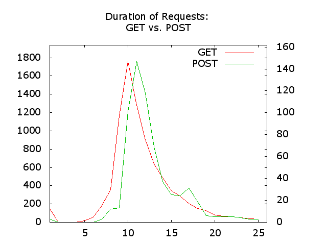
References
License / Copying / Further use

This work is licensed under a Creative Commons Attribution-NonCommercial-ShareAlike 4.0 International License.
Changelog
- 2018-04-13: Update title format (markdown); rewordings (Simon Studer)
- 2017-12-17: Fixed several links
- 2016-10-10: Fixing small issues
- 2016-07-15: Apache 2.4.20 -> 2.4.23
- 2016-07-15: Apache 2.4.20 -> 2.4.23
- 2016-04-18: Fixing small issues
- 2016-03-10: Translated to English